Learning to Play Settlers of Catan with Deep Reinforcement Learning
In recent years RL has attracted a lot of attention due to the extremely impressive results that have been achieved in games such as Go
As a way to teach myself about RL, a couple of years ago I built a simulator and trained an agent
I ended up deciding that an interesting game to try would be "Settlers of Catan" - a hugely popular board game that has sold over 35 million copies worldwide that I personally enjoy playing with friends. This is a game with a complex state/action space (placing roads/settlements, playing development cards, trading/exchanging resources etc), as well as being 4-player with some hidden information and every game requiring a large number of decisions. Without doubt it is more complicated than Big 2, but I thought that it is still significantly more accessible than an RTS like Starcraft 2. So whilst I recognised that this was going to be a serious challenge I thought it was perhaps possible that I could make some progress.
The plan for this article is to give a detailed overview of the approach I took, the difficulties that arose and the results I've been able to get so far. Whilst I haven't yet been able to get to the point where the trained agents perform at a super-human level, there has still been definite learning progress and the results are quite interesting. Hopefully this article will be interesting to anyone who has an interest in deep RL (or Settlers of Catan) - and in particular I hope it will be useful to anyone who is planning to try and apply RL themsevles to a new, reasonably complicated environment.
Before we get going, it is worth pointing out that others have made some attempts to apply RL to Settlers of Catan. However, as far as I'm aware these all either required the use of some pre-defined heuristics
The first step I took was to build a simulator implementing all of the rules of Catan. Whilst there are already well established and open-source code implementations available - in particular JSettlers - I decided to build my own from scratch for a number of reasons. Firstly, the only experience I have making a game simulator is with my previous Big 2 project, which was quite a while ago and quite a bit simpler, so I thought it would be quite fun to code everything myself. But more importantly I wanted something written in Python that I had full control over. Particularly since I don't have much Java experience, I felt like certain things (such as figuring out the action masks representing which actions are available in a given state) would be much simpler if I'd written my own simulator and understood everything about it in detail without having to dive into the JSettlers source code. Writing it in Python also has the advantage of making it much easier to integrate with the RL algorithm.
Another key reason is that I wanted to keep open the option of building forward-search methods (e.g. Monte-carlo Tree Search) to use with the trained RL agent. This requires being able to save and reset the state of the simulator and I assumed this would probably be a bit of a pain using JSettlers (although I admit I haven't properly looked into this in detail so it might be possible). Finally, developing the environment specifically with RL in mind just allows you to structure everything in a way that makes applying RL easier (unfortunately I have a lot of experience in trying to apply RL to simulation software that wasn't designed for RL, which can be quite frustrating!).
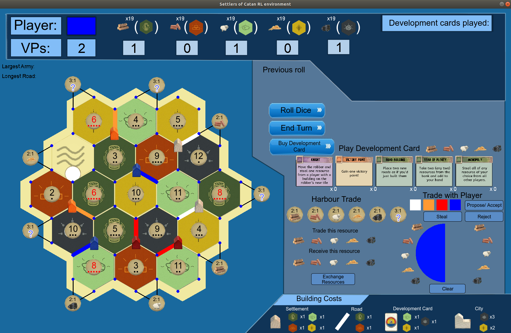
The main drawback was that obviously this ended up being a pretty big job in itself, especially since I decided early on that I needed to make a GUI and human-playable mode so that I could actually play against any agents that I trained (it's also really useful for debugging). I used PyGame for this, which is nice and simple to get started with but does have some limitations and things that make it a bit annoying to work with. But for my purposes it was just about good enough, and I was actually quite happy with how it ended up looking (all the code, including the simulator, is available on Github).
Other than the GUI and ensuring that the base game logic was all correct, one of the main things that the simulator needed was a way of representing which actions are available to an agent in any given state. As we will explore in the next section, Settlers of Catan has a complicated action space with a wide variety of different action types that an agent can play, not all of which are possible depending on the current state of the game. In fact, in a typical state a vast majority of all possible actions an agent could take will not be allowed (e.g. if they don't have the resources to build a settlement, or there are no valid corners to build on). As such, to train the agent in an efficient manner it is crucially important to mask out invalid actions. The alternative - i.e. allowing the agent to take invalid actions but ensuring they don't have any affect on the environment - is incredibly inefficient, since the agent would waste a huge amount of time trying out actions that do nothing.
The key ideas to deal with the action space was to use a combination of different action heads for different types of actions, and to have the simulator generate a corresponding set of masks that prevent invalid actions from ever being selected. The use of different action heads imposes some structure on the action space, which in principle should make training more efficient.
Let's start by considering the most naive approach we could take and think about some potential issues that may arise. An obvious idea would be to simply define a fixed set of actions and then have the neural network policy output a fixed size vector of probabilities over all of these possible actions (masking out all the actions which are unavailable in the current state - i.e. manually setting the probabilities to zero). So for example, you could have the first 54 components of the vector corresponding to placing a settlement on each of the 54 corners of the board, whilst the next 72 could correspond to placing a road on any of the 72 edges of the board, etc.
Whilst this is probably not too bad for placing settlements and roads, the first issue that arises is that some of the other available actions are a bit more complicated to model. For example, let's consider playing the "Year of Plenty" development card. When the card is played the user is allowed to choose two resources to take from the bank. This effectively makes it a composite action - you choose to play the card and you also need to select the two resources to receive. If we want to treat this as a single decision it means that there need to be 15 separate entries in the fixed size set of actions - one for each combination of resources (we can assume the order of resources is irrelevant). But this means that the network will have to learn about each of these 15 possibilities separately. So when it receives feedback from playing one of these actions (e.g. let's say that the agent went on to receive more reward than usual, so it wants to increase the probability of playing that action again in a similar situation), there is no direct mechanism that will lead to that feedback impacting the probabilities of the other 14 (quite similar) actions. Given that playing a "year of plenty" development card is quite rare anyway this will mean that the agent is likely to require an infeasible amount of experience to learn about all of these different possibilities independently. The alternative would be to break this down this down into three separate decisions - with one of the entries in the fixed size vector representing playing the card, and five entries corresponding to selecting a resource. Then once the card has been played, the simulator could mask out all actions that do not correspond to selecting a resource for the next two decisions. I suspect this might be preferable in this situation, however it's still not ideal because you have turned what should be a single action into three. Additionally, the network will need to be provided with information about the context of each of the three decisions its making and calculating the correct action masks for each decision can get a little tricky. These problems are exacerbated even further when we think about how to model trading resources.
This gives some motivation for using multiple action heads. The idea is that the first head will output the action type whilst the other heads will output the quantities that are needed for the particular type of action which is selected. These outputs can then be combined into "composite" actions (when necessary). So if we go back to the "year of plenty" development card example - the first head will output the action type (play development card), then a development card head will output the development card type (year of plenty), and then two separate resource heads will output the two desired resources. This allows us to break down the composite decision into components, with each head free to focus entirely on its part of the decision (conditional on the input from the other heads - so for example the resource heads will be given the context of the decision made by the development card head). This has the advantage of allowing composite actions to be chosen as part of a single "decision" (one pass through the neural network), as well as potentially allowing for much better generalisation since the feedback from the action (in terms of estimated values/advantages) can be applied to each head separately. In the example mentioned, this means that playing the "year of plenty" card can be reinforced directly via the development card head regardless of which resources are actually chosen - which in principle should make the learning process significantly more efficient.
As a quick technical aside, the RL algorithm used (PPO
So we get the log probability of the composite action simply by summing the log probabilities of each relevant action head!
Having said all of this, using multiple action heads in this way is not trivial, and I will now try and explain in detail how this was implemented in practice. To get started with, I broke the basic actions down into the 13 types described in the table below:
The reinforcement learning agent will operate at the level of these base actions - i.e. each decision the agent makes will correspond to one of these action types. In general a player's turn will be made up of multiple of these base actions which they can take one after the other until they choose the "end turn" action (at which point control will pass to the next player).
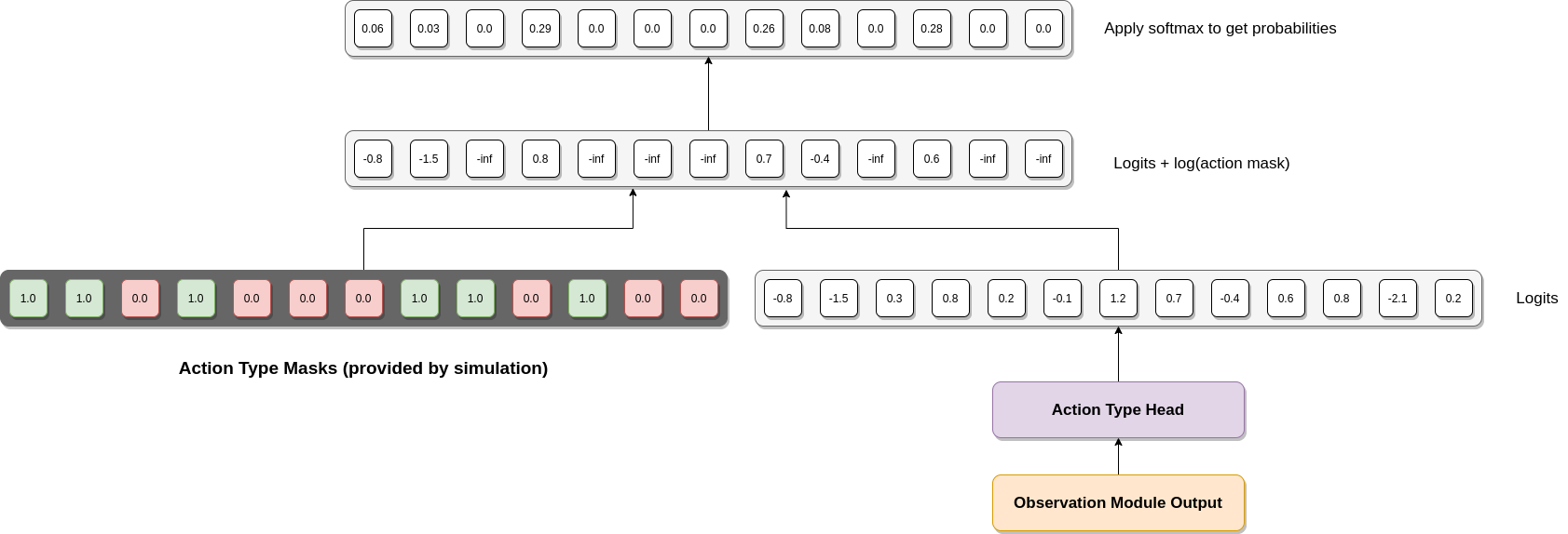
As mentioned, the first action head is the one that chooses the type of action (one of the 13 listed above). I think it's worth going through in full detail how this head works before diving into more detail about how the other heads work/ how they are combined together.
The diagram below illustrates what happens. The output from the "observation" module (see next section) is provided as input to the action head (a two layer fully connected neural network), which outputs a vector of logits (one for each action type). Before turning this into a probability distribution over actions we apply the relevant action mask provided by the simulation. This is a vector of 1s and 0s representing which types of actions are possible in the current state (valid actions are represented by 1.0, invalid actions by 0.0). What we do is then take the log of these action masks (so valid actions are mapped to 0, whilst invalid actions are mapped to negative infinity) and add them to the logits. For the valid action types this will have no effect, but invalid actions will be set to minus infinity. This means that when the softmax is applied their probabilities will be set to zero, ensuring that invalid actions are never selected.
The next head is the "corner" head, which outputs a categorical distribution over the 54 possible corner locations where settlements can in principle be placed (or upgraded to cities). This is only required for the "place settlement" and "upgrade to city" action types (the same head is used for both and the action type is provided as input to the head along with the output of the observation module - so it knows whether it's placing a settlement or upgrading to a city). For all other action types the output of this head will be masked out (note that because we have to train on large batches of data this head always has to be processed, but the output can be masked out depending on the action type chosen). The simulation environment also provides separate action masks for each of the two action types this head can be used for to mask out any invalid actions.
After that we have the "edge" head, which outputs a distribution over the 72 possible edges a road can be placed on. This is obviously only used for the "place road" action type, and is masked out otherwise. The input is simply the observation output (it doesn't explicitly need to receive the action type output because it is only ever used for one type of action and masked out otherwise).
The third head is the "tile" head - giving a distribution over the 19 tiles. This is only ever used with the moving the robber action type. Again its only input is the observation module output.
The fourth head in the "development card" head - giving a distribution over the 5 types of development card (obviously cards that the player does not own are masked out). This is only used with the play development card action type, and again its input is the observation module output.
The fifth head is the "accept/reject deal" head, which is used when the player has been offered a trade by another player. In this case it takes as input both the observation module output and a representation of the proposed trade and outputs a 2-dimensional categorical distribution over the two options (accept or reject).
The sixth head is the "choose player" head. This is used for the steal action type (after the player has moved the robber and is allowed to steal a resource from a player) and also for the propose trade action type (in this case the output of this head will be combined with the outputs of the "trade: to give" head and the "trade: to receive" head). So in this case the head takes both the observation module output and the action type (steal or propose trade) as inputs and outputs a categorical distribution over the available players (ordered clockwise from the decision-making player).
The next two heads are "resource" heads. The first resource head is used for the exchange resource action type (representing the resource to trade) and the play development card action type but only when the development card is "monopoly" or "year of plenty", otherwise it is masked out. The second resource head is also used for the exchange resource action type (representing the resource to receive) and the "year of plenty" development card. As such, these heads take the observation module output, the action type and the development card type (if applicable) as inputs, and output a categorical distribution over the 5 resources in the game.
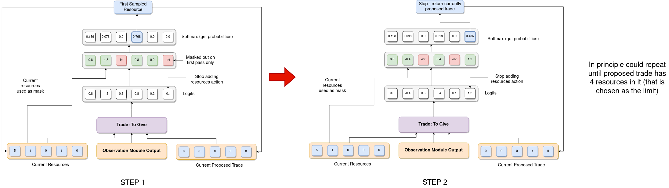
The next two heads are the most complicated since they represent proposing the resources for a trade. The first of these outputs the resources the player is proposing to give away. The main difficulty here is that in general the trade to be proposed can contain a variable number of resources (on both sides) and so the agent needs a way to be able to choose a variable number of resources (ideally without just considering every possible combination of resources as different actions). The way I decided to approach this was by using a recurrent action head where each pass of the head outputs a probability distribution over the five possible resources plus an additional stop adding resources action. The output of this head is then sampled and added to the "currently proposed trade". Provided the action chosen wasn't the "stop adding resources" action, this updated proposed trade is then fed back into the same action head along with the other inputs (the observation module output and the player's current resources, which is also updated based on the previous output). This allows the agent to iteratively add resources to the proposed trade as many times as it wants (although in practice I set a maximum of 4 resources on each side of the trade). The player's current resources can also be used here as the action mask for this head - ensuring the player never proposes to give away resources they do not actually have. The basic procedure for how this head operates is shown in the figure below:
The secondary trading head operates in a very similar way, with the main difference being that it doesn't need to use the player's current resources as an action mask because this head models the resources the player is proposing to receive. In fact, for simplicity I decided not to use action masks on this head at all - so player's can request any number of resources from the player they are proposing the trade to even if they do not have those resources (in which case they will have to reject the trade). On reflection this is potentially quite inefficient, and especially as learning to trade is potentially one of the most challenging things for an RL Catan agent to learn I do wish I'd done this differently (the reason it's not straightforward is that the mask to use would depend on the output of the "choose player" head which gets a bit fiddly, especially when processing a batch of data. However, given that I'd already gone to the effort of making e.g. the mask used for the corner head depend on the output of the "action type" head this was definitely quite doable).
So the full composite "propose trade" action consists of the output of the action type head, the choose player head and the recurrent "trade: to give" and "trade: to receive" heads.
The final head is the "discard resource" head. Whenever a player has 8 or more resources and a 7 is rolled (by any player) they must discard resources until they only have 7 left. I did consider using a recurrent head here as well - so that a player could choose all of the resources to discard in a single decision (if they had to discard more than one resource). I didn't do this in the end primarily because I thought it would probably be easier to use in the forward search planner (see later section) if each action only involved discarding a single resource, but also because it was a lot simpler to implement this way. The downside is that obviously this leads to the agent having to potentially carry out a large number of decisions if they get into a situation where they need to discard a lot of resources. I'm still unsure as to whether this was a good decision, and this is one of a number of design choices I would have liked to evaluate more thoroughly if I had access to more computational resources!
So bringing this all together I decided to build a little interactive demo of how the action heads work together! This ended up taking way longer than I had anticipated because my Javascript skills were extremely rusty but I was pretty happy with the results. The basic idea of the app is to show the flow of information through the whole action module when the agent is making a single decision. The orange boxes represent inputs which are passed into the actual action heads (fully connected neural networks, represented by pink boxes). The action heads each output logits (represented as little squares) which are then masked out by a particular action mask (shown as red boxes). In general these can depend on the output of any of the earlier action heads. After taking the softmax (not explicitly shown) the resultant probabilities are sampled to choose an action output from that head (represented by the blue boxes). The outputs of a given head can then in principle be used as part of the input for one of the later heads, or be used to pick the particular action mask used at a later head. As mentioned before, note that all action heads are sampled whenever the agent makes a decision, even when they are not relevant for the particular action type chosen. Although this may seem wasteful, it is necessary in order for us to be able to process multiple inputs in parallel in batches. Any outputs that are not relevant simply have their contribution to the overall action log probability masked out to zero (in the app this is represented by making the outputs from heads which are not needed for the sampled action type transparent).
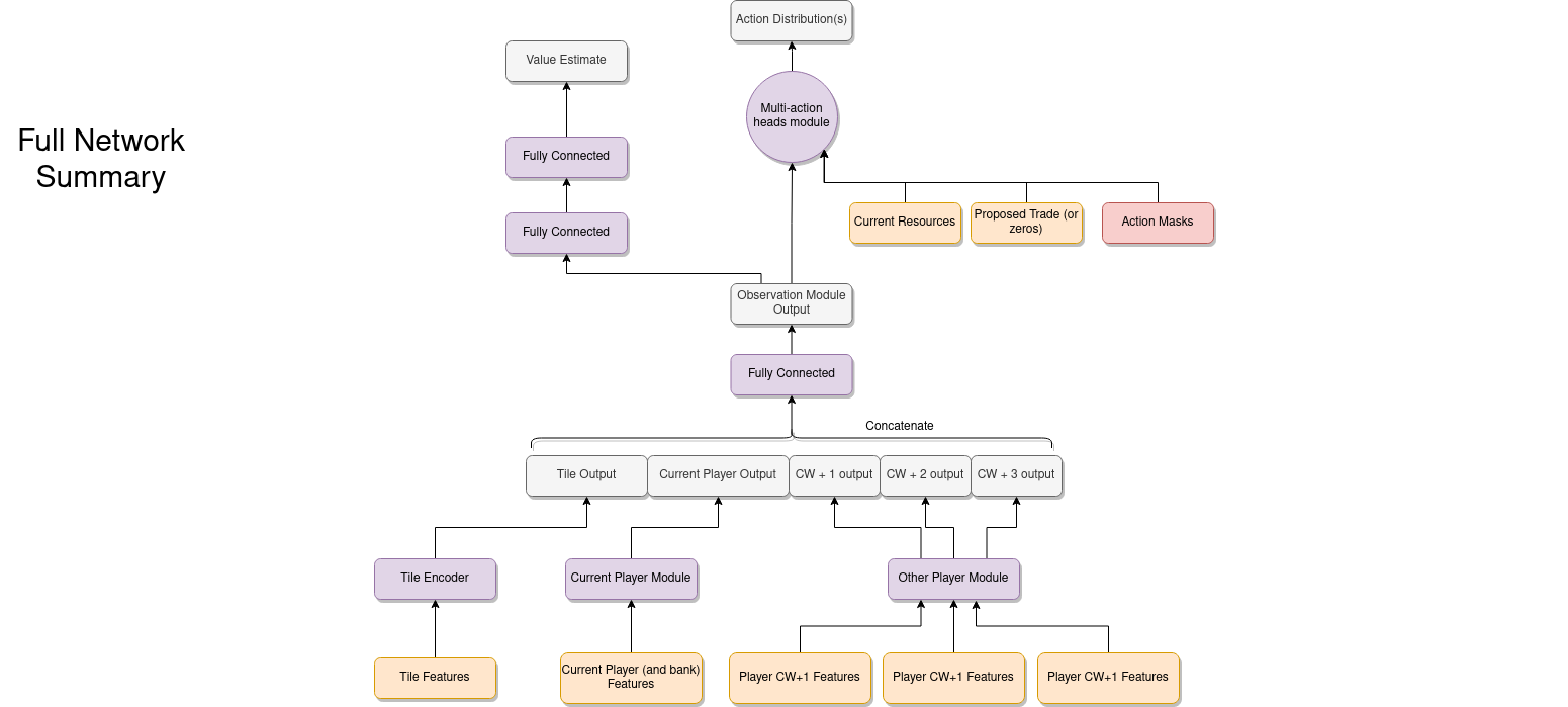
Just as important as the action space is the observation space. The main objectives here are to represent the current state of the game in a way that is appropriate to be processed by a deep neural network and then design the actual architecture of that neural network so that the agent is able to learn effectively.
To get started with this I decided to break the game state, or "observation", into three main parts. Firstly, features associated with each tile on the board are extracted and stacked together. The first of these is the tile's value - represented as a one-hot encoded vector (essentially each possible value is given its own dimension and the vector is zero everywhere except in the dimension corresponding to the actual value which is set to one). Using a one-hot encoded vector instead of just giving the neural network the actual value as a number is crucial because it is makes it much easier to learn a representation that treats each of the possible values differently (particularly as there is no simple ordering of values - 6 and 8 are "best" because they get rolled the most often, whilst 2 and 12 are "worst").
The feature vectors for each tile come out being 61-dimensional. All of these individual tile feature vectors are then fed into a multi-head attention mechanism
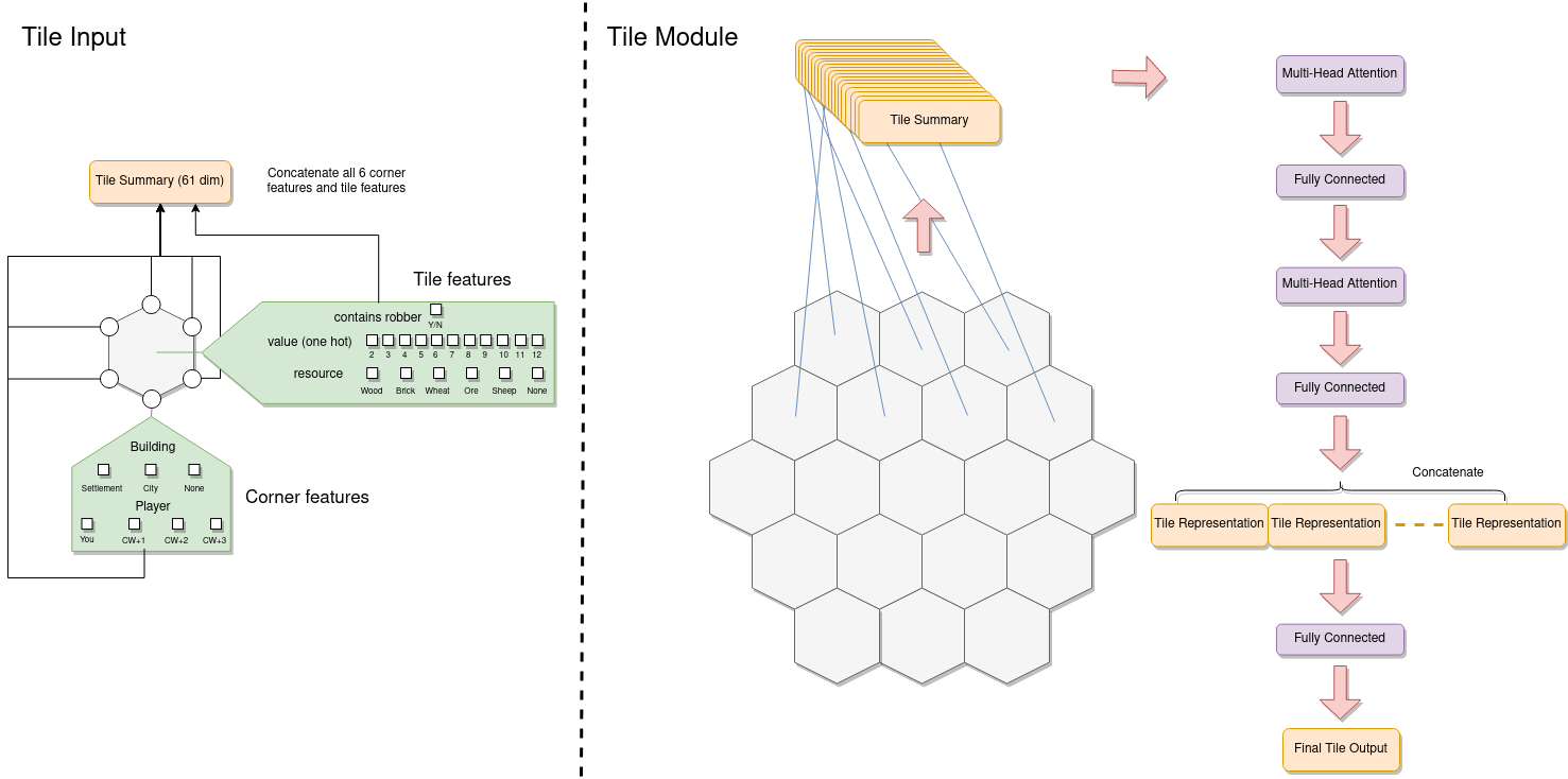
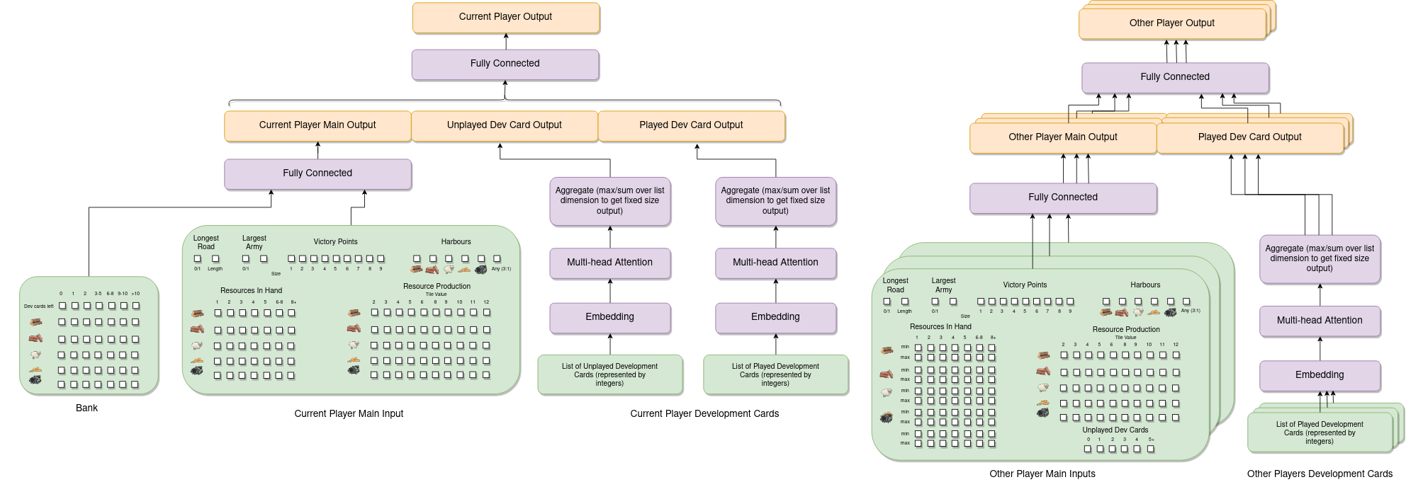
Next we need to summarise the current state of each player in the game in more detail. For the "current" player (i.e. the player making the decision) we generate a fixed size vector of features. These include two inputs for the longest road (whether the current player has the longest road and the normalised length of their current longest road) and two inputs corresponding to the largest army (whether they currently have the largest army and the current size of their army - i.e. how many knight development cards they've played). Next there is a one-hot encoding of the current number of victory points the player has, and then a feature vector representing which harbours (if any) they currently own. Finally, a summary of both the current resources the player has as well as the production for each resource is included. For each resource a vector is given representing the number of that resource the player has. For simplicity I decided to limit this to a separate entry for 1, 2, 3, 4 or 5 of that resource, and then two additional entries for 6-8 and 8+ (if the player has none of that resource then obviously all entries will be zero). This is injecting a small amount of prior knowledge that the agent probably doesn't need to distinguish between cases where, say, it has 8 wood and situations where it has 10 wood, because that is a lot of wood! To give information about the resource production a vector for each resource indicating the number of settlements that provide the player with that resource when a given value is rolled is provided. So for example, if a player had a settlement on a wood tile with value 6 then the entry in the wood vector corresponding to 6 would be set to 1 (or 2 for a city, and if there are multiple settlements this could be even higher - so this vector does not have values constrained to just 0 and 1).
This, along with a vector summarising the amount of resources/development cards left in the bank is passed into a fully connected layer. The main thing missing here is information about the player's development cards, which is dealt with separately because the player can both own and have played a variable number of cards. As such, both the cards the player has in their hand at the moment and the cards that they've played before are encoded as variable length lists of integers. These are then passed through an embedding layer and then into a multi-head attention mechanism. After the attention mechanism the representations of each card are aggregated into a fixed size vector by taking the sum over the list dimension for all of the cards. This allows the agent to learn a fixed-size representation of a potentially variable length sequence of development cards, and is concatenated with the "main" current player output before being fed into another fully connected layer.
The final thing that the agent needs to know about is information about the other players. For each player a feature vector similar to the one for the current player is constructed. The key difference is that the other player's resources/development cards are hidden (but a lot of things can be tracked - e.g. everyone knows when a player gathers a resource from someone rolling a particular number). To deal with this, I set up the environment in a way that keeps track of the minimum and maximum number of each resource that each player could have given the publicly available information. The feature vector for each other player then includes both of these. Additionally the feature vector includes information about the number of unplayed development cards, but nothing else. However the development cards that that player has played in the past is publicly available information, and this is processed with an embedding and multi-head attention layer in the same way as the development cards of the current player.
The feature vectors for each of the three other players are all processed in parallel by the same fully connected layers for improved efficiency, before eventually being concatenated together along with the tile module output and current player output. This concatenated output is fed through another fully connected layer before being designated as the "observation module output" (so it is this output that is used as the main input to each of the action heads described in the previous section).
A lot of the features and architecture choices made here could have been done differently, and so I make no claims that this is definitely the best way to do things. Additionally as I have said, I simply don't have the computational resources available to experiment with a lot of the choices to see how they empirically effect the performance. Nevertheless, I am reasonably satisfied that the approach I've taken and the choices I've made are at least sensible (and as we shall see they do lead to some clear learning progress). One other option that I initially experimented with was including an LSTM which I thought might be useful because there is some hidden information which means the current observation does not capture everything about the current state of the game. In the end I decided to remove this because (a) it didn't seem to make much difference in my initial quick experiments and (b) it's a bit tricky to integrate properly with the forward search method in a fully satisfactory way.
Having described in detail how to deal with the complex action/observation space that Settlers of Catan has, the next thing is to actually implement the RL algorithm. I decided to go with PPO as the base RL algorithm for a number of reasons:
As a general rule it is a bad idea to start implementing a deep RL algorithm from scratch. They are notoriously sensitive to seemingly minor implementation details that can have a huge impact on performance and trying to figure out exactly what small thing you've got wrong can be a painful experience. As such, I started from this excellent Pytorch implementation, but obviously still needed to make some fairly significant modifications to get it working with this environment.
One of the key differences between Settlers and the more standard environments that PPO is applied to is that it is a four-player game - which presents a number of challenges. Firstly, it makes everything non-stationary in the sense that the optimal policy depends significantly on the policies of the other players in the game. This means effectively that the environment changes over time as the opponents being played against learn to improve as well, which can often make the training process less stable. Additionally, it means that the agent really needs to learn a policy that can perform well against a variety of different opponents, and we must be careful to ensure it doesn't overfit to a particular set of opponents. To address this, I decided that when gathering a batch of data to train on only one of the four players would be "actively" controlled by the policy being trained, whilst the other three players would be controlled by earlier versions of the policy chosen at random (well, not completely at random - I decided to bias it so that more recent policies were more likely to be chosen). Note that because PPO is an on-policy RL algorithm the experience gathered by these other policies cannot be used in the training update. This does make the whole process significantly less data efficient but that is just a cost that has to be accepted to use PPO here, I think.
One technical detail that arises because of this is worth discussing. Most standard open-source implementations of PPO implement what I will call "synchronous" PPO. In this case, multiple CPU processes each containing their own copy of the environment run in parallel and are controlled by a main process. This main process has a single copy of the current policy, usually stored on a GPU, and receives observations from all of the processes at once. It then runs these through the policy as a batch, getting the actions for each environment before broadcasting them out to the relevant processes. Each process then runs the action given through its environment and sends back the next observation. This means that each process is effectively locked in step, and the main process can only get the next batch of actions once every process has finished and returned the next observation.
The approach has some advantages and some disadvantages. The main advantages are that it only requires a single copy of the policy on the main process which means less memory is needed and also that it allows for all of the observations to be processed as a batch on a GPU. For large policies and particularly when dealing with image observations when the forward pass of the network is still significantly expensive this can lead to a substantial boost in performance. The key disadvantage, however, is that if there is significant variation in the amount of time it can take to execute actions then processes can spend a lot of their time idly waiting until all of the processes finish (and note that this gets worse with the more processes that are running in parallel). The basic idea is shown on the left in the diagram below - if any of the processes have a particularly slow step (red) then this can have an effect on slowing down all of the other processes.
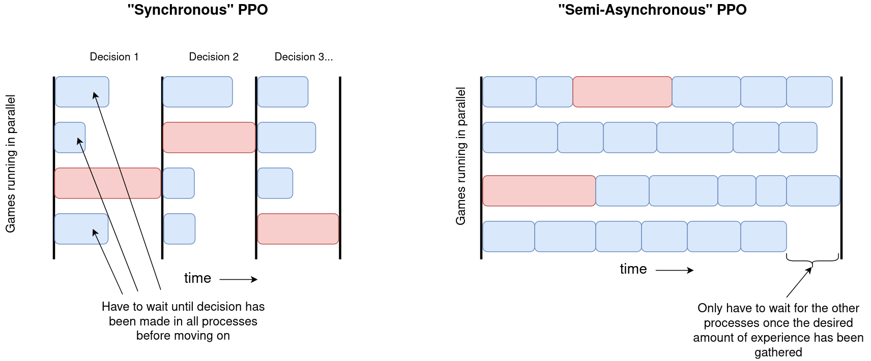
However, ultimately for our purposes here "synchronous" PPO just doesn't work. The main reason is that the time between each decision that the active agent has to make can vary wildly. This is because after the final decision of a player's turn they generally have to wait until all three of the other players have had their turns (each consisting of multiple decisions in general) before they get another decision to make. Addtionally, we want each process to have different opponents on them to ensure there is enough diversity in each batch so we don't strongly overfit. This requires that each process contains its own copies of the opponents policies. This meant that the PPO implementation needed to be modified to be "semi-asynchronous".
What this means in practice is that each process contains four policies - one for each player in the game (in fact due to memory constraints during training each process actually contained 5 games, with the same policies controlling the players for each of these). The "main" process sends out a request for each process to gather a specified amount of experience and each process is left to run independently until it has gathered this data. The processes all have to wait for the other processes to finish at the end (which is why I call this "semi-asynchronous" rather than fully asynchronous), but not after each decision, which is obviously far more efficient for our purposes here. The main process then combines all of this experience into a single large batch of data to train the main policy on. Then it selects new opponent policies for each process and broadcasts these out along with the updated main policy, before requesting each process to gather a new batch of data.
The only real downside of this approach is that each process has to have its own copy of multiple policies, which can get quite memory intensive. Also generally this means that when acting you won't be able to utilise a GPU to run batches of forward passes in parallel, but this isn't so bad as really it is the backward passes required during training that are most expensive and benefit the most from a GPU.
Beyond this the only other significant/relevant changes I made to the base PPO implementation was to implement value function normalisation and to allow for returns to be recomputed after each optimisation epoch (see table below). This is something that was suggested in this
Other than these changes, the other key decisions to make are what values of the hyperparameters used in PPO to use. Even though PPO is one of the more robust RL algorithms, it is still well known that the performance can be significantly impacted by the choices of hyperparameters. Frustratingly there are no definitive rules that can guide which hyperparameter values will work well on a given environment and whenever possible the best approach is to simply run hyperparameter sweeps over at least some of the key parameters. However, in this case this simply isn't feasible and so I had to rely on my experience with other environments to effectively make some "informed guesses". The main hyperparameters considered along with a description and some justification (where possible) for the values chosen are detailed in the table below.
| Hyperparameter | Description | Value chosen | Comment |
|---|---|---|---|
| Number of Processes | The number of processes that run in parallel when gathering a batch of experience. Each process runs each of its assigned environments to gather a fixed number of decisions made by the agent being trained. | 128 | Generally speaking, the more processes the better. But obviously there are constraints based on available resources (number of CPUs and memory). Also as each process has to wait for all other processes once it has gathered its specified amount of decisions a very large number of processes can lead to significant idle time. This is why when training with a very large amount of available compute it's usually better to implement a fully asynchronous version of PPO. |
| Number of Environments per Process | The number of games each process has going on at once. Each game is controlled by the same set of neural networks (one active player for which we are gathering data, and three networks using an earlier versions of the policy). Note that they can still control different players in each game (e.g. the colour/order in which they play is still different in each game). | 5 | Ideally we want to be gathering data from as many games as possible so that each batch contains a wide variety of situations for the agent to be in (to help protect against overfitting). It would probably be preferable for each game to be on its own process so that each game is being played against a different set of opponents, however because each process has to have 4 copies of a neural network on this leads to large memory consumption. Having multiple games per process increases the variety of experience gathered whilst reducing the amount of memory required. |
| Number of Decisions (per Environment per Batch) | The number of decisions the agent being trained (i.e. the agent with the most recent policy) should make in each game on each process. | 200 | So the total batch size (in terms of the number of decisions made) is 128 x 5 x 200 = 128000. |
| Number of Epochs of Optimisation per Batch | The number of "epochs" (i.e. full passes through the batch of data) of optimisation. That is, given the full batch of data, an epoch of optimisation involves dividing the data up (at random) into a number of minibatches. Each of these minibatches is then passed through the policy being trained and used to calculate the gradients of the networks parameters with respect to the PPO loss. | 10 | I have seen values between 3 and 10 used for different environments. Ideally this is a hyperparameter that should be tuned. |
| Number of Minibatches per Epoch | The number of minibatches each epoch is broken up into (so each epoch consists of this many gradient updates to the model). | 64 | So each minibatch is made up of 128000 / 64 = 2000 samples. Whilst I think this is reasonable, I have to say I'm not completely sure. |
| Discount Factor (\(\gamma\)) | How much future rewards are effectively discounted when estimating values (i.e. the sum of future rewards is taken to be \( \sum_{t'=t}^T \gamma^{t'-t} r_{t'} \) rather than just \( \sum_{t'=t}^T r_{t'} \) ) | 0.999 | Having a value slightly less than one helps with stability, even with finite length episodes. However given that we care about optimising over fairly long time horizons we don't want it to be too much less than 1. Possibly we could have gotten away with a slightly lower value (say 0.995 or 0.997), which might have helped with stability. A rough rule of thumb is that you want the time horizon over which you're interested in (\(\text{num_steps} \)) to satisfy \( \text{num_steps} \sim \frac{1}{1-\gamma} \), although I'm not sure if this holds to the same extent when the main reward you care about is sparse and at the final step so I tend to verge on the cautious side of making \( \gamma \) a bit larger in those situations. |
| Generalised Advantage Estimation (GAE) Parameter (\(\lambda\)) | Without going into full detail (see the original paper |
0.95 | This is a very commonly used value across many environments. I have found with experiments on other environments that actually other values can work slightly better, but without performing expensive hyperparameter sweeps this is always a good default value. |
| Clipping Parameter (\(\epsilon\)) | A parameter used in PPO to control how much the policy is able to change in a single update. Imposing this (soft) constraint means that the policy cannot change too much in a single update and therefore cannot completely overfit to the current batch of data that's been gathered. | 0.2 | Often a parameter that is explored in a hyperparameter sweep. Values are usually between 0.1 and 0.3 for most environments but 0.2 is a common value and a reasonable default. |
| Recompute Returns after Each Epoch | In the standard PPO implementation GAE is applied once per batch just after it's been gathered. This gives a set of estimated values, returns and advantages associated with each state in the batch and these are kept fixed throughout the whole update. However, after each minibatch both the policy and the value network have changed slightly. This means the value/advantage estimates are suddenly out of date. It's not really feasible to recompute the returns after each minibatch update, but we can recompute them after each epoch at least. | True | It has been shown that this can often give a reasonable boost in performance and so is worth including by default. |
| Entropy Loss Coefficient | A coefficient managing the strength of the contribution of the policy's entropy to the overall loss function being trained on. The idea is that the larger this is the more the policy will be encouraged to explore. | 0.01 | I did initially consider annealing this down over time, so that gradually the agent has less pressure to ensure high entropy over its actions, but I decided not to in the end. |
So, how did this all work out? For the final run I ran an experiment for roughly a month on a 32-core desktop machine with 128GB of RAM and a GTX3090 GPU. The answer is basically - it definitely learned some stuff and absolutely got better over time, but it still doesn't feel close to the standard of a good human player (having said that, I did come dangerously close to losing a game against it the other day). This is slightly disappointing, but perhaps not really surprising - we know that current deep RL algorithms are greedy and require a huge amount of experience to play games such as Chess/Go to the standard of a human - and ultimately the amount of compute I threw at it is miniscule in comparison to projects such as AlphaGo and the OpenAI DOTA 2 bot. Another potential reason for the slow progress is that I did not have any human data to start from, which can make a massive difference. Certainly both AlphaGo and AlphaStar made use of a large dataset of human gameplay to train an initial policy to imitate before running the RL algorithm (although I believe this wasn't done with AlphaZero).
Having played a few games against the trained agent (plus forward-search, see next section), I can give a rough outline of some of the behaviours I've observed. The first thing is that it definitely has not yet mastered trading, which is not really surprising given that this is one of the more complicated aspects of the game. The agent still wastes a lot of time proposing trades that the other player isn't actually able to accept (I definitely regret not masking out these actions as invalid), and more often than not if the trade is possible it's also massively in its own favour and so no rational agent would accept. As such, a majority of the allowed trades that get proposed immediately get rejected, although not always. I think the fact that the agents still sometimes accept trades completely against their interests (even with low probability) encourages the agents to continue to propose unfair trades - because there is effectively no cost to doing so and sometimes they get a nice benefit. As such, if you do want to play against the trained agent (available on the Github repo linked to in the contents) I would recommend turning off trading, because frankly it's a bit tiresome having to constantly reject stupid trades.
With the forward-search included I've found that generally the initial settlement placements seem fairly reasonable, which is promising and definitely suggests the agent has learned something about the relative value of different positions on the board. However in the later game I have definitely seen some questionable road/settlement placements which don't make a lot of sense, so clearly there is a lot of room for improvement.
Another interesting thing I've noticed is that the agents rarely get caught holding more than 7 resources when a 7 is rolled, and so rarely have to discard any resources. So they definitely have learned that having to discard resources is bad, however they sometimes will do quite stupid things to get rid of them (e.g. exchanging 4 stone for 1 stone...). In terms of things like moving the robber, the agents usually do this when they have the chance and will always steal a resource, which is good. However they do sometimes move the robber to a tile which doesn't really benefit them (e.g. if they also have a settlement that gets blocked by it).
To look at the results and learning progress more quantitatively, I carried out a couple of evaluation runs looking at the agent at different points in the training process playing against agents slightly earlier in the training process. The final experiment ran roughly 3500 full updates (each update corresponds to multiple epochs of optimisation on a batch of experience of 128000 decisions - so roughly 450 million decisions in total). Every 100 updates I played a number of games (1200) with the current policy at that point against 3 copies of the policy at either 125 updates before or 250 updates before (obviously this choice is somewhat arbitrary). If all the policies were completely equal we would of course expect each policy to win 25% of the games, so we can look to see what fraction of games are won by the "current policy" when it plays against multiple copies of an earlier policy. If this is consistently above 25%, it gives a good indication that the policy is still learning and improving. The results of this evaluation are plotted below.
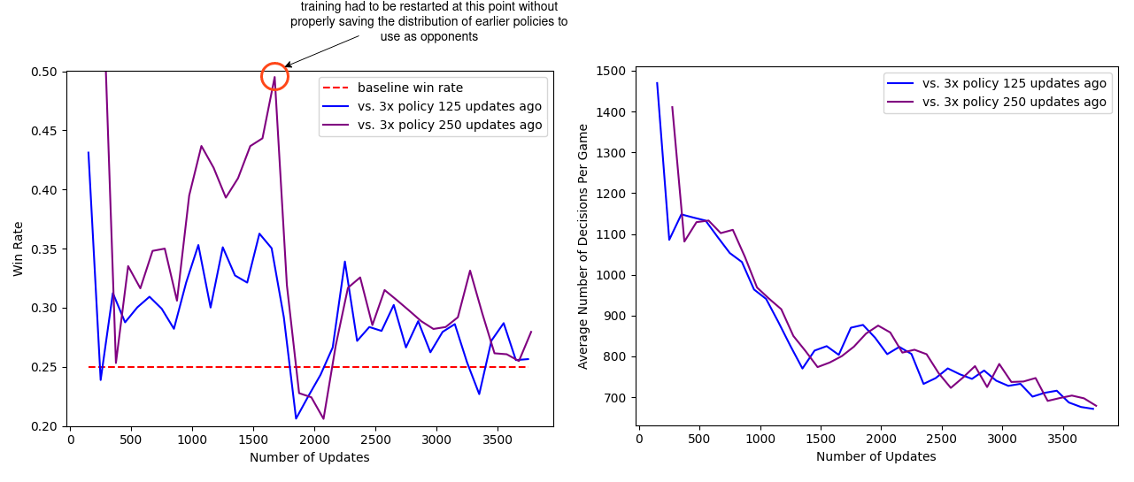
We can see that initially there is significant learning progress, clearly above the baseline winrate. It is also reassuring to see that the winrate against the policies 250 updates ago is generally above the winrate against the more recent policies (125 updates ago). Unfortunately about half-way through the experiment the computer crashed and training had to be reinitialised. Annoyingly I realised I hadn't set things up properly to reinitialise the distribution of opponent policies that were being sampled and I only had copies of the previous policies every 25 updates. This meant I had to try and construct an ad-hoc distribution based on the available policies that was significantly different from what would have been in the experiment when it was running. It certainly appears like this had a big impact - with the win rate briefly falling below the baseline. However, eventually things stablised and we got back to a situation where the policy seemed to be improving again, although interestingly not as quickly as before. This might just be a natural slowing down in the speed of improvement, although it is slightly suspicious/strange that we never get back to the same rate of improvement we were seeing before the crash.
Also plotted is the average total number of decisions made per game (here the total includes decisions by all four players). Up until a certain point it is reasonable to assume that shorter game lengths correspond to agents that are learning to improve (as they are learning to win the game more quickly), although obviously we wouldn't expect this trend to continue indefinitely. As such, it is quite promising that even towards the end of training there is still a clear trend down towards shorter games, suggesting that the agents are still improving.
Another thing which is quite interesting to look at is how the agent's certainty about its decisions changes throughout training. From the evaluation runs carried out above I saved the probability of each action that was actually selected (for each relevant of the relevant action heads). We can then use these to gain some insight into how often the agent chooses to play different action types and how this changes throughout training.
Firstly we can focus just on the action types that the agent chooses to play (taking the probability just from the action type head). Each plot below shows the type probability vs. the number of action types that were available when the decision was made. Note that this is the probability of that action type when that action type was actually selected, which means that the values will be somewhat biased to be larger, but can still give an interesting insight into what's going on.
As would be expected, we can see that early on during training there is a wide range of type probabilities for each action type. However as training goes on, the certainty with which the agent plays certain actions (in particular placing a settlement, upgrading to a city and moving the robber) increases a lot. Whilst this certainly makes some sense, the fact that the probabilities get so close to 1 suggests that perhaps the agent is overconfident in its choices.
We can also look at the probability of some of the other heads. Below are plots for the probability of choosing a particular settlement location (when that settlement location is chosen), choosing a particular road placement, a particular city placement and a particular placement for where to move the robber. For all of these we see that the agent gradually becomes more confident about its decisions throughout training - although it would appear at different rates for different action types.
An often overlooked detail about some of RL's greatest successes is that many of them require search on top of the RL policy in order to actually surpass human performance (this is certainly true for AlphaGo and AlphaZero). This usually takes the form of a "Monte Carlo Tree Search"
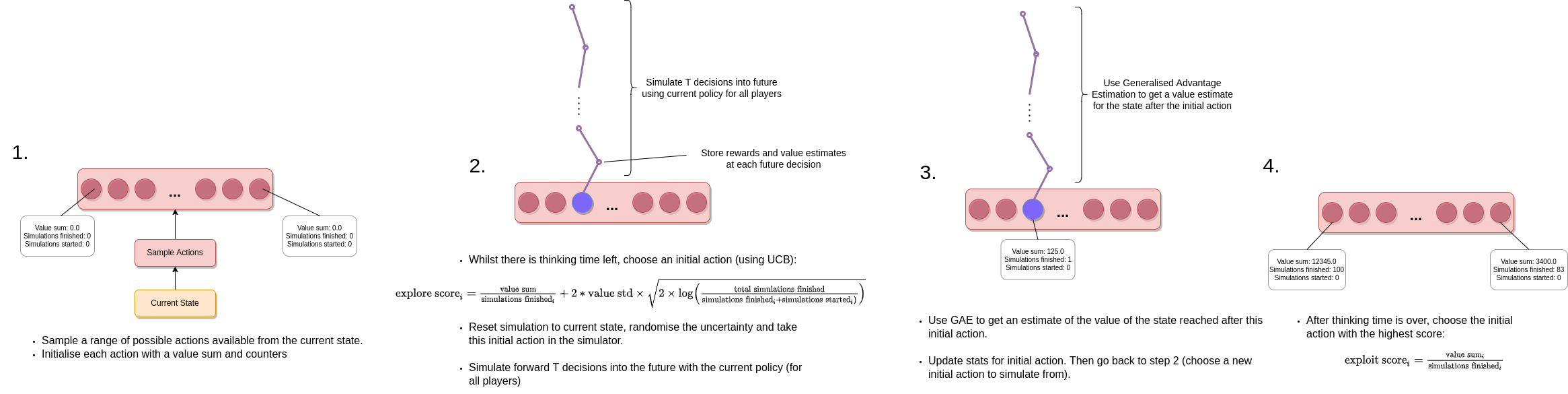
Rather than perform a proper tree search I instead decided to just search over a set of sampled actions available in the current state, making use of the current policy to run monte carlo simulations of how the game could play out for \(T \) steps into the future. That is, the search process itself is only conducted over the actions available from the root node (the current state), and then rollouts are carried out into the future using the current policy for all of the agents to make decisions. For each rollout we can then use generalised advantage estimation to estimate the value of the state that's reached after the initial action we're considering, which can then be stored along with the visit count for that initial action. This can then be used to choose which initial action is chosen for the next simulation to run forwards using UCB1 (in the same way that actions are chosen in MCTS, except here we are only performing this search at the root of the tree of actions).
To be able to parallelise this search, we make use of the approach outlined in the "WU-UCT" paper
One of the nice things about the action head architecture being used is that it's possible to pick actions conditional on a given action type. This allows us to sample a wide range of initial actions, even if they are very unlikely to be picked by the policy be default. In particular, I ensured that any action type that was available is always sampled at least once (and possibly more). Also, the action masks can be modified to ensure the policy never samples the exact same action twice. Additionally, I decided that in the initial placement phase of the game it would be a good idea to consider all actions available (and give the agent more thinking time than usual, since these are particularly important decisions). The full logic of how the actions to consider for each decision are sampled is contained here.
A couple of other important details are worth mentioning here. The first is that this forward search method (and indeed any search method like this that performs search with the actual environment rather than a learned model of the environment) requires that the simulator can save its current state and then reload it later. This is one of the reasons I was keen to implement my own simulator, so I had complete control over doing this. The other thing is that Settlers of Catan has some hidden information in the sense that you don't necessarily know exactly what resources/development cards the other players have. This is relevant in the forward search because you can't (or at least shouldn't) just reset the state of the simulation exactly because the player making the decision doesn't actually know everything about the current state of the simulation. As such, I had to implement a "randomise uncertainty" method, which randomises the other player's unknown resources/development cards (based on the best information the decision-making agent currently has).
To test this, I ran 100 games with one agent using this forward search method (32 processes in parallel, 10 second base thinking time per decision, using the final policy from training for forward simulations) against three copies of the final policy. The forward search agent won 47/100, showing that there is a clear improvement here over the RL agent alone.
In an ideal world, I would have liked to do something more similar to AlphaZero, where the forward search is used during training to collect experience and train. This can lead to a much stronger policy (as well as a much better learned value function), but requires an enormous amount of compute so just wasn't feasible. Additionally, it would definitely be interesting to look at a stronger MCTS search method that actually searches beyond just the root node (and so doesn't have to rely fully on the policy alone for future simulations) and see if this makes a signficant difference.
Overall this has been a really interesting project and I have learned a lot - particularly about how to deal with complex action spaces in RL. Whilst there is a part of me that is a bit disappointed that the final agent is still not at the level of a good human, the fact that it clearly learned some interesting behaviour and improved significantly throughout training is pretty cool, especially given the relatively modest amount of computational resources used.
One thing I think that I might have done differently if I were starting from scratch is to remove trading because I think that was probably a bit ambitious. Whilst I think the approach I took was interesting and could maybe work well if I could run some larger scale experiments, I think the fact that the agents waste so much time proposing stupid trades could have had a significant effect on training - and it might have been possible for the agents to learn more efficiently if this was just removed. Obviously trading is a big part of Catan, but even without trading it is still a very challenging game. At some point I may just start another training run with trading turned off to see if this is true or not, but atm I need my desktop for other things!
Anyway, I hope this article was interesting and potentially useful to anyone looking to apply deep RL to other environments. Please feel free to ask any questions in the comments below and I'll do my best to answer them!